Getting Started with rwanikani

Introduction

The rwanikani package provides a comprehensive R interface to the WaniKani API v2. WaniKani is a popular spaced repetition system for learning Japanese kanji, vocabulary, and radicals. This package allows you to programmatically access your learning data, progress statistics, and study materials.

Installation

You can install the development version of rwanikani from GitHub:

# devtools::install_github("jonocarroll/rwanikani")

Authentication

Before you can use any functions in rwanikani, you need to authenticate with the WaniKani API using your personal API token.

Getting Your API Token

1. Log in to your WaniKani account
2. Go to Settings > API Tokens
3. Generate a new API token with the permissions you need
4. Copy the token for use with this package

Setting Your API Key

You can set your API key in two ways:

library(rwanikani)

# Method 1: Set directly in R
wk_set_api_key("your-api-token-here")

# Method 2: Set as environment variable (recommended)
Sys.setenv(WANIKANI_API_KEY = "your-api-token-here")
wk_set_api_key()  # Will automatically use the environment variable

For security, it’s recommended to set the WANIKANI_API_KEY environment variable in your .Renviron file:

WANIKANI_API_KEY=your-api-token-here

Basic Usage

Let’s start with some basic examples of how to use the package.

Get User Information

# Get information about your WaniKani account
user_info <- wk_user()

print(paste("Username:", user_info$username))
#> [1] "Username: jonocarroll"
print(paste("Current Level:", user_info$level))
#> [1] "Current Level: 8"
print(paste("Subscription Active:", user_info$subscription$active))
#> [1] "Subscription Active: TRUE"

Get Subjects (Radicals, Kanji, Vocabulary)

# Get subjects for your current level
current_level <- user_info$level
subjects <- wk_subjects(levels = current_level)

print(paste("Number of subjects at level", current_level, ":", length(subjects$data)))
#> [1] "Number of subjects at level 8 : 180"

# Get only kanji subjects
kanji_subjects <- wk_subjects(types = "kanji", levels = 1:5)
print(paste("Number of kanji in levels 1-5:", length(kanji_subjects$data)))
#> [1] "Number of kanji in levels 1-5: 167"

# Get all subjects (warning: this might take a while and use many API calls)
# all_subjects <- wk_subjects(all_pages = TRUE)

Get Your Assignments

# Get all your current assignments
assignments <- wk_assignments()

# Get assignments that are currently available for review
available_assignments <- wk_assignments(
  available_at_before = Sys.time(),
  srs_stages = 1:8  # Exclude burned items (stage 9)
)

print(paste("Available reviews:", length(available_assignments$data)))
#> [1] "Available reviews: 500"

# Get assignments for specific levels
level_assignments <- wk_assignments(levels = 1:3)

Get Review Data

# Get recent reviews (last 24 hours)
recent_reviews <- wk_reviews(
  updated_after = Sys.time() - 24*60*60  # 24 hours ago
)

print(paste("Reviews in last 24 hours:", length(recent_reviews$data)))
#> [1] "Reviews in last 24 hours: 0"

# Get all reviews for specific subjects
subject_reviews <- wk_reviews(subject_ids = c(1, 2, 3))

Advanced Usage

Working with Review Statistics

# Get the 5 subjects with lowest accuracy (most mistakes)
wk_print_mistakes(5)
#> ℹ Fetching review statistics...
#> ℹ Loading subjects data from cache
#> ℹ Processing 1189 review statistics...
#> ✔ Found 5 subjects with lowest accuracy
#> === Subjects That Need More Practice ===
#> 
#> 1. この前 (The Other Day, Recently, In Front of This) - Meaning: 63% [Level 8 Vocabulary]
#> 2. 者 (Someone, Somebody) - Meaning: 67% [Level 8 Kanji]
#> 3. 向こう (Over There, Opposite Side, Other Side, Far Away) - Meaning: 67% [Level 8 Vocabulary]
#> 4. 全く (Completely, Entirely, Truly, Really, Wholly) - Meaning: 67% [Level 8 Vocabulary]
#> 5. 助ける (To Help, To Save, To Rescue) - Meaning: 67% [Level 8 Vocabulary]

# Or get the raw data for further analysis
mistakes <- wk_get_mistakes(10)
#> ℹ Fetching review statistics...
#> ℹ Loading subjects data from cache
#> ℹ Processing 1189 review statistics...
#> ✔ Found 10 subjects with lowest accuracy
head(mistakes)
#>      subject_id characters                                        meanings level object_type meaning_percentage
#> 1168       3457     この前       The Other Day, Recently, In Front of This     8  vocabulary                 63
#> 1144        690         者                               Someone, Somebody     8       kanji                 67
#> 1146       3428     向こう Over There, Opposite Side, Other Side, Far Away     8  vocabulary                 67
#> 1162       3454       全く     Completely, Entirely, Truly, Really, Wholly     8  vocabulary                 67
#> 1181       2997     助ける                     To Help, To Save, To Rescue     8  vocabulary                 67
#> 1187        687         決                                Decide, Decision     8       kanji                 67
#>      reading_percentage
#> 1168                 NA
#> 1144                 NA
#> 1146                 NA
#> 1162                 NA
#> 1181                 NA
#> 1187                 NA

# Find subjects with accuracy below a specific threshold
low_performers <- wk_get_mistakes(n = 20, percentage_threshold = 60)
#> ℹ Fetching review statistics...
#> ℹ No review statistics found
if (nrow(low_performers) > 0) {
  print(paste("Found", nrow(low_performers), "subjects with less than 60% accuracy"))
}

Study Materials and Notes

# Get your personal study materials (notes and synonyms)
# study_materials <- wk_study_materials(all_pages = TRUE)

# Filter study materials for specific subject types
kanji_materials <- wk_study_materials(subject_types = "kanji")

print(paste("Number of kanji with personal notes:", length(kanji_materials$data)))
#> [1] "Number of kanji with personal notes: 1"

Level Progression Analysis

# Get and display level progression summary
wk_print_level_progression_summary(wk_level_progressions(all_pages = TRUE))
#> ℹ Formatting 8 level progressions...
#> ✔ Formatted 8 level progressions
#> === Level Progression Summary ===
#> 
#> Total levels tracked: 8 
#> Levels completed: 0 
#> Levels passed (not completed): 7 
#> Levels in progress: 1 
#> 
#> Passing Time Statistics:
#>   Average days to pass: 25.5 
#>   Median days to pass: 21.2 
#>   Fastest level passed: 10.1 days
#>   Slowest level passed: 48.6 days
#> 
#> Individual Level Progress:
#>    Level 1 - passed in 13 days 
#>    Level 2 - passed in 10.1 days 
#>    Level 3 - passed in 24 days 
#>    Level 4 - passed in 21.2 days 
#>    Level 5 - passed in 13.7 days 
#>    Level 6 - passed in 47.8 days 
#>    Level 7 - passed in 48.6 days 
#>    Level 8 - in progress

Data Analysis Examples

Creating Summary Statistics

# Function to analyze your current progress
analyze_progress <- function() {
  # Get user info
  user <- wk_user()
  
  # Get assignments for current level
  current_assignments <- wk_assignments(levels = user$level)
  
  # Count assignments by SRS stage
  srs_counts <- table(sapply(current_assignments$data, function(x) x$data$srs_stage))
  
  # Get available reviews
  available <- wk_assignments(
    available_at_before = Sys.time(),
    srs_stages = 1:8
  )
  
  cat("=== WaniKani Progress Summary ===\n")
  cat("Current Level:", user$level, "\n")
  cat("Available Reviews:", length(available$data), "\n\n")
  
  cat("Current Level SRS Distribution:\n")
  stage_names <- c("Initiate", "Apprentice I", "Apprentice II", "Apprentice III",
                   "Guru I", "Guru II", "Master", "Enlightened", "Burned")
  for (stage in names(srs_counts)) {
    cat(paste(stage_names[as.numeric(stage)+1], ":", srs_counts[stage], "\n"))
  }
}

# Run the analysis
analyze_progress()
#> === WaniKani Progress Summary ===
#> Current Level: 8 
#> Available Reviews: 500 
#> 
#> Current Level SRS Distribution:
#> Initiate : 30 
#> Apprentice I : 2 
#> Apprentice II : 13 
#> Apprentice III : 3 
#> Guru I : 31 
#> Guru II : 22

Next Steps

This vignette covered the basics of using rwanikani. For more detailed information about specific functions, see their help pages:

?wk_user
?wk_subjects
?wk_assignments
?wk_reviews
?wk_review_statistics
?wk_study_materials
?wk_level_progressions
?wk_resets

Working with Kanji Similarity Data

The rwanikani package provides powerful tools for extracting and analyzing kanji similarity information from the WaniKani API.

Extracting Kanji with Similarity Information

# Get kanji table with similarity data using cached subjects
kanji_table <- wk_get_kanji_table(levels = 1:20, include_similarity = TRUE)
#> ℹ Loading subjects data from cache
#> ℹ Processing 707 kanji subjects...

# Show the structure
head(kanji_table)
#>    id  type kanji meanings                  readings level  similar
#> 1 440 kanji    一      One いち / いつ / ひと / かず     1         
#> 2 441 kanji    二      Two                 に / ふた     1         
#> 3 442 kanji    九     Nine      く / きゅう / ここの     1 467, 447
#> 4 443 kanji    七    Seven        しち / なな / なの     1         
#> 5 444 kanji    人   Person   にん / じん / ひと / と     1      445
#> 6 445 kanji    入    Enter        にゅう / はい / い     1      444

The similarity data comes directly from WaniKani’s API and includes visually similar kanji that might be confusing to learners.

Resolving Similarity IDs to Readable Format

The raw similarity data contains kanji IDs. You can resolve these to show the actual kanji characters and meanings:

# Get subjects data for similarity resolution
subjects <- wk_load_subjects_cache(levels = 1:20, types = "kanji")
#> ℹ Loading subjects data from cache

# Resolve similarity IDs to show kanji and meanings
kanji_resolved <- wk_resolve_similarity_details(kanji_table, subjects$data, format = "kanji_meaning")

# Find kanji with similarity data
similar_kanji <- kanji_resolved[kanji_resolved$similar != "" & !is.na(kanji_resolved$similar), ]

# Show first 10 kanji that have similarity information
if (nrow(similar_kanji) >= 10) {
  print("First 10 kanji with similarity data:")
  similarity_examples <- similar_kanji[1:10, c("kanji", "meanings", "level", "similar_resolved")]
  print(similarity_examples)
} else if (nrow(similar_kanji) > 0) {
  print(paste("Found", nrow(similar_kanji), "kanji with similarity data:"))
  print(similar_kanji[, c("kanji", "meanings", "level", "similar_resolved")])
} else {
  print("No kanji with similarity data found in levels 1-10")
}
#> [1] "First 10 kanji with similarity data:"
#>    kanji meanings level                   similar_resolved
#> 3     九     Nine     1            丸 (Circle), 力 (Power)
#> 5     人   Person     1                         入 (Enter)
#> 6     入    Enter     1                        人 (Person)
#> 8     力    Power     1 丸 (Circle), 九 (Nine), 刀 (Sword)
#> 9     力 Strength     1 丸 (Circle), 九 (Nine), 刀 (Sword)
#> 10    力  Ability     1 丸 (Circle), 九 (Nine), 刀 (Sword)
#> 21    大      Big     1                 太 (Fat), 犬 (Dog)
#> 22    大    Large     1                 太 (Fat), 犬 (Dog)
#> 24    山 Mountain     1                                   
#> 28    刀    Sword     2                         力 (Power)

Understanding Similarity Data

The similarity information helps identify kanji that are visually similar and commonly confused:

• Raw IDs: "717, 832, 1486" - WaniKani’s internal subject IDs
• Resolved Format: "氷 (Ice), 永 (Eternity), 泳 (Swim)" - Shows the actual similar kanji with their primary meanings

Different Similarity Formats

# Just show the similar kanji characters
kanji_only <- wk_resolve_similarity_details(kanji_table, subjects$data, format = "kanji")

# Keep the original IDs
ids_only <- wk_resolve_similarity_details(kanji_table, subjects$data, format = "ids")

# Full kanji with meanings (default)
full_format <- wk_resolve_similarity_details(kanji_table, subjects$data, format = "kanji_meaning")

Adding Custom Similarity Mappings

If you want to add your own similarity relationships:

# Define custom similarity mappings
custom_similarity <- list(
  "479" = "717, 832, 1486, 537, 913",  # 水 (water) similar kanji
  "481" = "505, 453",                   # 犬 (dog) similar kanji  
  "482" = "528, 1286, 794, 679, 1745"  # 王 (king) similar kanji
)

# Apply custom mappings
kanji_with_custom <- wk_add_similarity(kanji_table, custom_similarity)

# Then resolve to readable format
custom_resolved <- wk_resolve_similarity_details(kanji_with_custom, subjects$data)

This similarity data is particularly useful for:

• Study Planning: Focus on groups of visually similar kanji together
• Error Analysis: Understand which kanji you might be confusing
• Mnemonic Creation: Create memory techniques that distinguish similar kanji
• Practice Sets: Create targeted practice for commonly confused characters

Interactive Kanji Network Visualization

The rwanikani package includes powerful network visualization capabilities to explore kanji similarity relationships visually, inspired by language graph visualizations.

Creating a Kanji Network

# Create an interactive network centered on a specific kanji
network_plot <- wk_kanji_network(
  kanji_resolved,           # Your kanji data with similarity information
  center_kanji = "水",      # The kanji to center the network on
  max_depth = 5,           # How many degrees of separation to show
  interactive = TRUE       # Create an interactive plotly visualization
)

# Or use English meaning instead of kanji
network_plot <- wk_kanji_network(
  kanji_resolved,
  center_kanji = "Water",   # English meaning will be resolved to 水
  max_depth = 5,
  interactive = TRUE
)
#> ℹ Using kanji '水' for meaning 'Water'

# Display the network
network_plot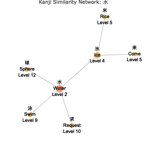

plot of chunk unnamed-chunk-16

Network Visualization Features

The network diagrams provide several powerful features:

Layout Options

# Force-directed layout (default) - organic, natural clustering
wk_kanji_network(kanji_resolved, "水", layout = "force")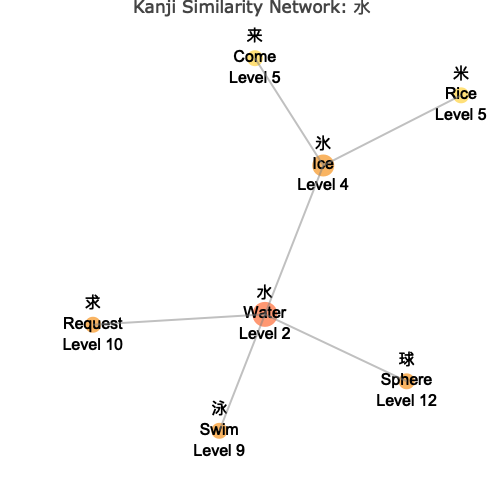

plot of chunk unnamed-chunk-17

# Circular layout - arranged in a circle
wk_kanji_network(kanji_resolved, "水", layout = "circle")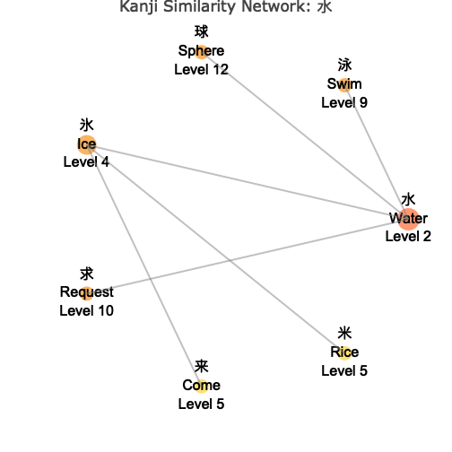

plot of chunk unnamed-chunk-17

# Tree layout - hierarchical structure
wk_kanji_network(kanji_resolved, "水", layout = "tree")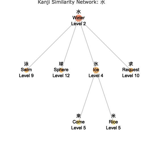

plot of chunk unnamed-chunk-17

# Grid layout - structured arrangement
wk_kanji_network(kanji_resolved, "水", layout = "grid")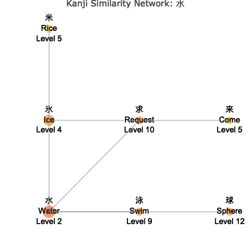

plot of chunk unnamed-chunk-17

Node Sizing Options

# Size by number of connections (default)
wk_kanji_network(kanji_resolved, "水", node_size_by = "connections")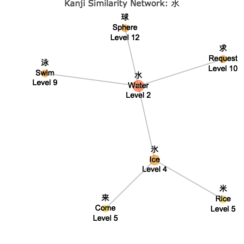

plot of chunk unnamed-chunk-18

# Size by WaniKani level (lower levels = larger nodes)
wk_kanji_network(kanji_resolved, "水", node_size_by = "level")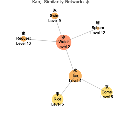

plot of chunk unnamed-chunk-18

# Fixed size for all nodes
wk_kanji_network(kanji_resolved, "水", node_size_by = "fixed")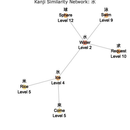

plot of chunk unnamed-chunk-18

Customization Options

# Show or hide meanings in node labels
wk_kanji_network(kanji_resolved, "Dog", show_meanings = TRUE)   # Show meanings (using English)
#> ℹ Using kanji '犬' for meaning 'Dog'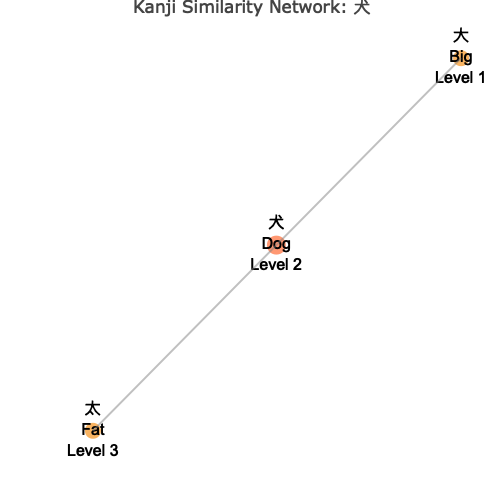

plot of chunk unnamed-chunk-19

wk_kanji_network(kanji_resolved, "犬", show_meanings = FALSE)   # Kanji only (using Japanese)

plot of chunk unnamed-chunk-19

# Create static ggplot instead of interactive plotly
static_plot <- wk_kanji_network(kanji_resolved, "水", interactive = FALSE)
static_plot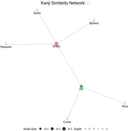

plot of chunk unnamed-chunk-19

# Control network depth
shallow_network <- wk_kanji_network(kanji_resolved, "水", max_depth = 1)  # Direct connections only
shallow_network

plot of chunk unnamed-chunk-19

deep_network <- wk_kanji_network(kanji_resolved, "水", max_depth = 8)     # 8 degrees of separation
deep_network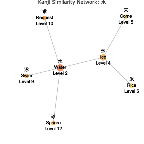

plot of chunk unnamed-chunk-19

Understanding the Network

The network visualization shows:

• Central Node: The target kanji you specified, highlighted in the center
• Connected Nodes: Similar kanji connected by lines (edges)
• Color Coding: Different colors indicate the “depth” or degrees of separation from the center
• Node Sizes: Vary based on your chosen metric (connections, level, or fixed)
• Interactive Features: Hover over nodes to see detailed information

Exploring Similarity Patterns

Networks help you discover interesting patterns:

# Explore highly connected kanji (kanji with many similar characters)
# These might be particularly confusing and worth extra study attention

# Find kanji at the center of similarity clusters
# Look for nodes with many connections in the network

# Discover unexpected relationships
# Sometimes kanji that seem unrelated are connected through similarity chains

Network Analysis Examples

# Compare different kanji networks
water_network <- wk_kanji_network(kanji_resolved, "水", max_depth = 4)
water_network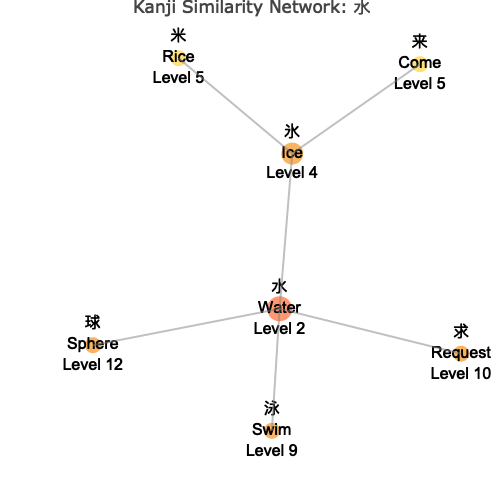

plot of chunk unnamed-chunk-21

circle_network <- wk_kanji_network(kanji_resolved, "丸", max_depth = 4)
circle_network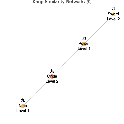

plot of chunk unnamed-chunk-21

valley_network <- wk_kanji_network(kanji_resolved, "谷", max_depth = 10)
valley_network

plot of chunk unnamed-chunk-21

# Create a comprehensive network for a complex kanji
complex_network <- wk_kanji_network(
  kanji_resolved, 
  center_kanji = "午",        # Language/word - likely has many connections
  max_depth = 5,             # Deep exploration
  layout = "force",          # Natural clustering
  node_size_by = "connections",  # Highlight highly connected kanji
  show_meanings = TRUE,      # Full information
  interactive = TRUE         # Interactive exploration
)
complex_network

plot of chunk unnamed-chunk-21

These network visualizations provide an intuitive way to understand kanji relationships and can help guide your study strategy by revealing clusters of visually similar characters.

You can also explore the package’s GitHub repository for more examples and to report issues or contribute improvements.